Competition judging is hard. Coming up with fair methods to select rankings is difficult, and it’s especially hard to design judging methods for large-scale events.

As an attendee of many hackathons, and as an organizer of HackMIT, I wanted to figure out a way to improve the quality of judging at hackathons and large-scale competitions in general. Sometimes, poor judging is a result of neglect or lack of organization. However, most judging methods themselves are inherently flawed. It’s possible to do a lot better.

When trying to design a good judging system, large-scale events in particular pose a unique challenge. Because the events are so large, no single judge can judge all the entries. In fact, at HackMIT, the average judge looked at only 5% of the projects. The challenge is to figure out what data to collect and how to combine the data to come up with good overall judging results.

Given the size of the event, the number of judges, and the amount of time there is for judging to take place, there is a fundamental limit on how much data it’s possible to collect. The question is: given the constraints, how do we produce the highest-quality judging results possible?

It turns out that we can radically change the judging model, and instead of having judges produce absolute scores, we can ask judges to perform pairwise comparisons. Using statistical inference methods, it’s possible to take data of this form and produce high-quality judging results.

The method of pairwise comparisons actually works pretty well in practice! We relied on this method for judging at Blueprint, HackMIT’s high school hackathon, and we’re thinking of using some form of this judging method starting from HackMIT 2015 as well.

Perhaps the most straightforward judging method is to have numerical scores and average them. It’s really easy to have judges assign numerical scores to each entry they judge, average the scores per entry, and rank the entries by average score.

Because this method is so easy to implement, it’s no wonder that it’s so common! The vast majority of events use something like this. However, this method is deeply flawed.

What does it mean when judge A gives entry X a 7/10, and judge B gives entry Y a 4/10? Does it mean that X was objectively better, or does it mean that judge B was particularly harsh? This is just one of the many problems with this method.

In some situations, it’s possible to improve the averaging approach by normalizing judges’ scores. This is a method that was used for judging MIT BitComp. In this system, to account for variations in judging, scores are normalized to have a mean of 0 and a standard deviation of 1. Given raw scores $x_1, x_2, \ldots, x_n$ from a single judge, we can compute normalized scores $x_i'$ by computing:

In the expression above, we have:

This is a step in the right direction. However, the approach is still flawed. For one, given the way that the numbers are for a lot of these large events, individual judges look at a tiny fraction of the entries. Normalizing judges’ scores could harm good entries, and it could also give an undeserved boost to bad entries.

Judging by assigning explicit numerical scores is inherently flawed. Assigning numerical scores to entries is not a task that people are good at! The following XKCD comic illustrates this phenomenon:

Numerical scores are nonsense to begin with. Even then, it’s especially bad when judges don’t have a global view of all the entries and only see a tiny percentage of entries. And with current systems, judging results are dependent on the order in which entries are judged. Judges look at one entry at a time, so when judging the first entry, they have no context and nothing to compare it to when assigning a score. After judging many entries, a judge’s outlook may change. Judging results should be independent of the order in which entries are judged! And judges can’t just go back and adjust scores — after judging several entries, they all start to blur together.

People are much better at making comparative judgements than determining absolute scores for options, and there’s a good amount of psychology and economics research to back up this claim¹. Pairwise comparison is the way to go for obtaining high-quality judging results.

It’s easy to understand the advantages of this approach by considering examples. Try rating emacs on a scale of 1-10. Now think about whether vim is better than emacs (sorry, I couldn’t resist).

When collecting pairwise comparison data, we do have to be a little careful. Even though we won’t necessarily have comparison data between every pair of entries, we do not want disjoint sets of entries that are never even indirectly compared to each other. Ensuring that we have good data, we can use information from the comparisons to determine a global ranking.

The method of pairwise comparison has other nice properties as well. Luce’s choice axiom states that the probability of selecting one item over another from a pool of many items is not affected by the presence or absence of other items. This is a nice property to have when judges see a small percentage of the entries — taking this independence property into account can allow us to develop better models.

Pairwise comparison is clearly the right way to measure the quality of entries. The tricky part is how to turn the measurements into judging results.

Before designing a model, it’s necessary to think about the form and representation of the results of many pairwise comparisons. We need to keep in mind that any given pair of entries may be compared with each other zero or more times, and that judges may have conflicting opinions about the comparative quality of entries.

The results of a pairwise comparisons between entries $e_1, e_2, \ldots, e_n$ is a multiset of tuples where the element $(e_j, e_i), j \neq i$ represents a single judging decision where entry $e_i$ was judged to be better than entry $e_j$.

We can also think of the measurements as a directed graph on $n$ nodes $e_1, e_2, \ldots, e_n$, representing the entries, having nonnegative integer edge weights, with edge $(e_j, e_i)$ having weight $w_{ij}$ equal to the number of times entry $e_i$ was judged to be better than $e_j$, so arrows point to better entries.

It’s also useful to consider a matrix representation of the data that follows naturally from the graph representation — we have a matrix $S$ with nonnegative integer entries, where $S_{ij}$ is equal to the number of times entry $e_i$ was judged to be better than $e_j$.

After we have a representation for our measurements, we can start thinking about how to translate comparisons into a ranking. It’s natural to think about finding a topological sort of the comparison graph. Informally, a topological sort would translate to a ranking that none of the judges disagree with. Unfortunately, in general, a topological sort will not necessarily exist, because the comparison graph could be cyclic.

Instead, we can consider a slightly different problem, finding the best possible ranking that we can in terms of some cost function. We are given a weighted directed graph $G = (V, E)$ with edges $(v_i, v_j)$ having weight $w_{ij}$. We can define a permutation of the nodes, $\sigma : V \rightarrow \{1, 2, \ldots, \vert V \vert\}$. Then, we can define backward edges as a function of the permutation, $E_B(\sigma) = \{(v_i, v_j) \in E \mid \sigma(v_i) > \sigma(v_j)\}$. We can define the cost of a given permutation as the sum of the weights of the backward edges:

We can then define the optimal ranking:

This method is pretty good. Informally, it represents finding a ranking that the least number of judging decisions disagree with. However, the algorithm doesn’t really take into account much about the nature of judging entries.

Also, there’s another issue — this is an NP-hard optimization problem! We can prove this via a simple reduction from the minimum feedback arc set problem, one of Karp’s 21 NP-complete problems, by setting all edge weights to 1.

We can look to psychology research to find good models for reasoning about paired comparison data. We turn to probabilistic choice models, using Thurstone’s statistical model of judgements, a widely accepted model that will allow us to derive interval scale measurements from which we can extract rankings.

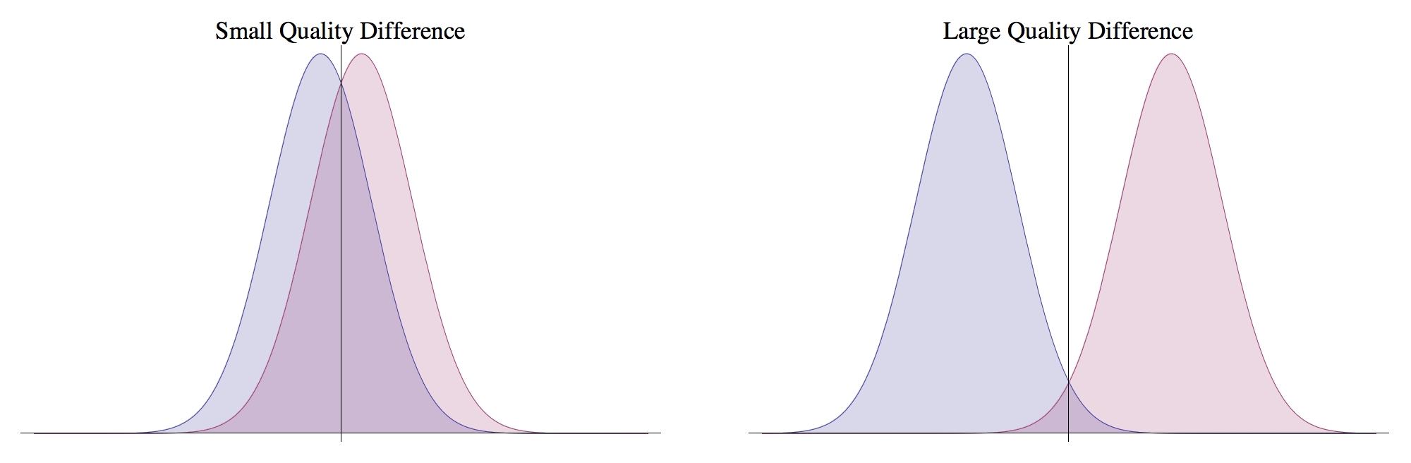
Thurstone’s model assumes that the quality of every choice is a Gaussian random variable. The model dictates that when a person judges the relative quality of two options, they sample from each of the corresponding quality distributions, and they choose the option with the higher measured quality. This is a pretty nice property in modeling the real world — when two options are very different in terms of quality, it’s easy to pick out the better one; however, when options are very similar in terms of quality, there will be a much smaller difference in the probability of choosing one over the other.

An option’s true quality is the mean of the corresponding Gaussian. Given whatever data we have, if we can figure out the means of the Gaussians, we will have relative scores for every option, so we’ll be able to determine a global ranking.

As an example, consider two options with Gaussian random variables $X$ and $Y$:

Their corresponding probability density functions are:

In the above expression, $\phi(z) = \frac{1}{\sqrt{2 \pi}} e^{- \frac{1}{2} z^2}$, the standard normal probability distribution function.

Given this information, we can compute the probability that a judge chooses a given option:

We have that $X - Y$ is a Gaussian random variable. We assume zero correlation in our model:

We can now compute the probability that $P(X > Y)$:

In the above expression, $\Phi(z) = \int_{-\infty}^{z} \phi(t) \, dt$, the standard normal cumulative distribution function.

We can simplify our model by setting $\sigma_X^2 = \sigma_Y^2$, and without loss of generality, we can let $\sigma_X^2 = \sigma_Y^2 = \frac{1}{2}$, so that we have $\sigma_{XY}^2 = 1$. This makes the math a little cleaner.

We hold that there exist true $\mu$s corresponding to each option, and given our data, we want to determine the most likely parameters for the model. We can construct a maximum likelihood estimator to do this.

First, we consider the case with a single pair of options, X and Y. Let $x$ be the number of people who chose option X, and let $y$ be the number who chose Y.

We can define the likelihood of measurements $x$ and $y$ given our data $\mu_{XY}$:

When maximizing, equivalently, we can calculate the log-likelihood, because the logarithm is strictly monotonically increasing:

Now, we can move on to constructing a maximum likelihood estimator for finding all the parameters. Here, it is convenient to consider the matrix representation of the judging decisions. Recall that we have a matrix $S$ where $S_{ij}$ is the number of times entry $i$ was preferred over entry $j$.

We can apply the maximum likelihood result from above. We note that the $\log {x + y \choose x}$ terms are constants given our data, and we recall that $\mu_{XY} = \mu_X - \mu_Y$. We can define the global maximum log-likelihood:

If we consider using a maximum a posteriori estimator, we can assume that option values were drawn independently from a normal distribution and use Tikhonov regularization, which will result in a higher-quality estimate. We can obtain this solution by solving the following convex optimization problem:

To make good use of our statistical model and inference algorithm, we need to make sure we have good data. We need to make sure that we have enough comparisons between pairs so that we can come up with a good global ranking, so we want to make sure we end up with a connected graph.

A good way to dispatch judges is to have them judge a sequence of options and compare each option with the previous one. This results in $n - 1$ data points from $n$ evaluations by a judge.

What good is fancy math unless it’s actually being used?

After implementing the algorithm and doing a good amount of modeling and analysis, the HackMIT team decided to use this as the judging method for Blueprint, our high-school hackathon.

Because of time constraints, our data collection method was a bit hacky, using a Twilio app to collect comparison data from judges. Running the algorithm involved me copying logs from the server, running data through a Python script, running a convex optimization routine written in MATLAB, and interpreting the results in Python! Even though the interface was… suboptimal, the algorithm was fully implemented, and it ended up working really well!

In case anyone wants to try experimenting with real-world data for personal use, here is anonymized data from the rookie division, consisting of 235 comparisons for 37 teams, and here are our results.

Here is a graphical representation of the comparisons that were made. In the graph, the nodes represent teams, and an edge from node X to node Y represents at least one judge choosing Y over X. Essentially, it’s the comparison graph with edge weights hidden:

Many judging methods that are commonly used at competitions are inherently flawed because of their use of absolute scores assigned by the judges. The method of paired comparisons is a much more natural system to use, and it can be used to obtain high-quality judging results.

We used this paired comparison method at Blueprint, and it worked out well for us. We’re thinking of using some variant of this method of judging starting from HackMIT 2015. I’d love to see this method being used at more competitions, because it’s likely to lead to higher quality results, and it could also lead to increased transparency in judging, which would be great.

For this method to be really easy for anyone to use, there needs to be an easy way of collecting paired comparison data and running the optimization algorithm. When I have some time, I’m thinking of working on a web app to make this whole process really easy, so that anyone will be able to use this judging method without having to think about the math or write a single line of code.

Update (11/12/2019): The judging system has been open sourced (as of September 2016) and has been successfully used at dozens of events.